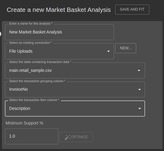
Create a new Market Basket analysis
Simply click the “plus” icon next to “Market Basket” in the left-hand naviation menu.

Then complete the simple form. Only two fields from a transactional data source are required - items being sold (SKU or Description) and an identifier to group multiple items into “baskets” (e.g. invoice numbers, sales order numbers, receipt numbers etc)
Identify your data source
| Field | Requirements |
|---|---|
| Connection | An existing connection. To create and manage connections, see Creating and Managing Database Connections |
| Table | An existing table or view in your data source. |
Typical ERP data sources will have Order Detail or Invoice Detail tables suitable for this analysis. POS data will also contain transaction datasets.
You may need to transform your data prior to analysis, or you may already have “analytic-ready” data prepared for reporting. If you have transformed and cleaned your data sufficient for generating reports, you likely already have good data for analytics - any further transformation will be handled automatically.
Choose analysis data fields
Market Basket analysis requires only two key pieces of data in your data source.
| Data element | Requirements |
|---|---|
| Transaction Grouping | Typically this will be an Invoice or Order number, basket identifier or other such field that groups multiple line-items into a single logical transaction. |
| Transaction Item | This could be an SKU (Stock Keeping Unit), or a more descriptive text field of the item. Often a data warehouse will use a Product Dimension to provide different levels of granularity for items - some experimentation may be required to see what works well with your own data. SKU fields are sometimes too detailed - they may have many different values for variants of the same product (size, color etc) and this can weaken the power of the analysis when you would consider any of the variations equivalent in terms of making a recommendation to a customer. |
Provide model input parameters
| Parameter | Requirements |
|---|---|
| Minimum Support % | An item must appear in at least this percentage of overall transactions to qualify for analysis. Higher values yield fewer, potentially more significant rules, although they may overlook subtle associations. Lower values produce a greater number of rules, which can make it difficult to identify the most relevant associations. The default setting is 1%, which serves as a solid starting point unless you have a very limited number of products in your catalog (in which case, a higher percentage may be appropriate). Conversely, if you have a huge product catalog, you might need to set a lower percentage to see any rules at all. |
| Optimize | Coming Soon |
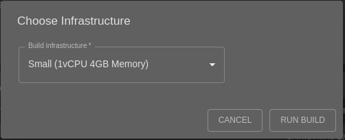
Choose a build infrastructure
See Build Infrastructure for details on the infrastructure provisioned for building the analysis.
Create the analysis
Once all fields are completed, you will see a previous of the data that you can use to sanity check that the correct fields are chosen. Click “Save and Fit” to continue.
Fitting
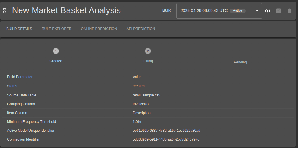
After clicking “Save and Fit”, you then select the infrastructure to deploy. A summary of the analysis is then displayed along with its status.
It may take a few seconds, a few minutes, or even a few hours, depending on data size to fit (or build) the model that provides this analysis.
The page will refresh automatically as the status moves from Created, to Fitting, to Fitted.
You may navigate away from this tab, or the whole application, without interrupting the build.
Assess the rules generated by the analysis
The “Rule Explorer” tab will become available once a model has been fitted (built).
Rules are displayed as an association between a set of items on the left and another set of items on the right. A rule implies that transactions which contain the items on the left will tend to also contain the items on the right. The left hand side is often referred to as the “antecedent” and the right as the “consequent”, and the strength of the association can be assessed by lots of different metrics.
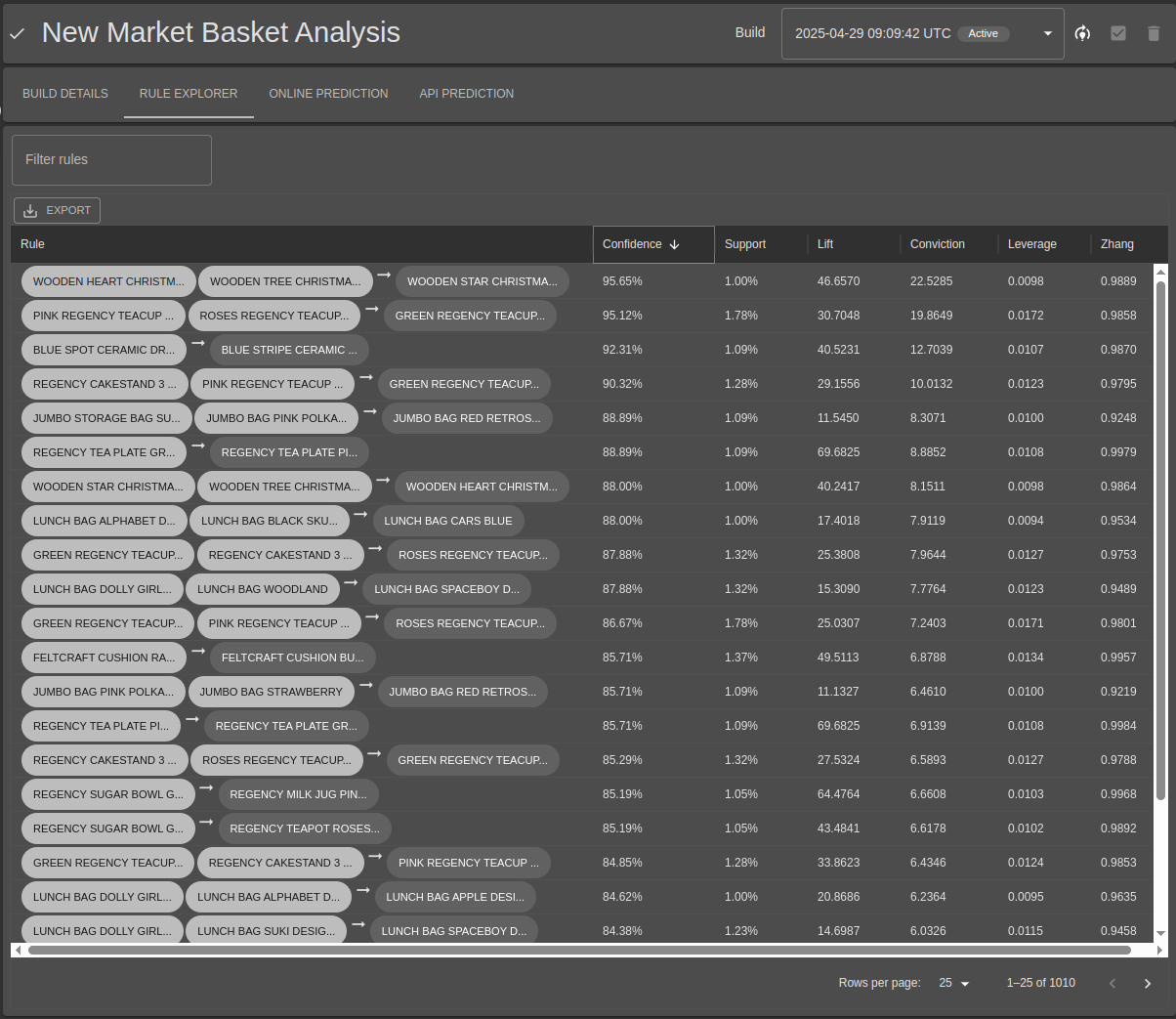
By default, rules are sorted by the highest “confidence” score and are unfiltered. To only display rules that contain a specific subset, enter text in the “Filter Rules” box and the rules will be narrowed down to items that contains that text.
The rules can be assessed by the following metrics.
| Metric | Descrition |
|---|---|
| Confidence | The confidence of a rule X->Y is the probability of seeing Y in a transaction given that it also contains X. The confidence for X->Y is different than the confidence for Y->X. The confidence reaches its maximum value of 1 if X and Y always occur together and never on their own. |
| Conviction | A high conviction value for X->Y means that Y highly depends on X (but not necesarily the other way around!). In the case of perfect confidence scores, this approaches infinity. Similar to lift, if items are completely independent, the conviction is 1. |
| Leverage | Leverage computes the difference between the observed frequency of A and C appearing together and the frequency that would be expected if A and C were independent. A leverage value of 0 indicates independence. |
| Lift | The lift metric for X->Y measures how much more often X and Y occur together than we would expect if they were statistically independent. If X and Y are independent, the Lift score will be exactly 1. A value or 2 would mean you are twice as likely to see X and Y in the same transaction as seeing either of them on their own. |
| Support | Support is used to measure the abundance or frequency of an itemset in the data source. It is the percentage of transactions that contain all of the items in the rule, whether on the left or right hand side. Rules that don’t meet the minimum support threshold specified when creating the model are dropped. |
| Zhangs Metric | Measures both association and dissociation. Value ranges between -1 and 1. A positive value (>0) indicates Association and negative value indicated dissociation. |
Association rules metrics are computed by the mlxtend library - formulae can be found on their documentation page
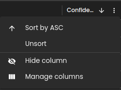
You may change the sort field or add/remove displayed columns by clicking the column header menu:
Re-fit the model on the latest available data
The data available via the configured data source may be constantly changing as new transactions are recorded. You may re-fit/re-build the underlying model for a given analysis without having to fill out all of the information again. Simple click the “Re-fit on latest data”  icon next to the drop-down list of available builds.

You may also set the Active model or delete a particular build. For more information on what the active model refers to, see Manage Existing Analysis Models .
Make predictions
While the Rule Explorer is good for manually reviewing rules, Online Prediction specifically returns suggested items given some already chosen items. It uses confidence to find and color-code suggested items. Add one or more Given/Current items to get started. Selecting many given items may return no suggested items as the number of rules with that specific combination is quickly filtered away.
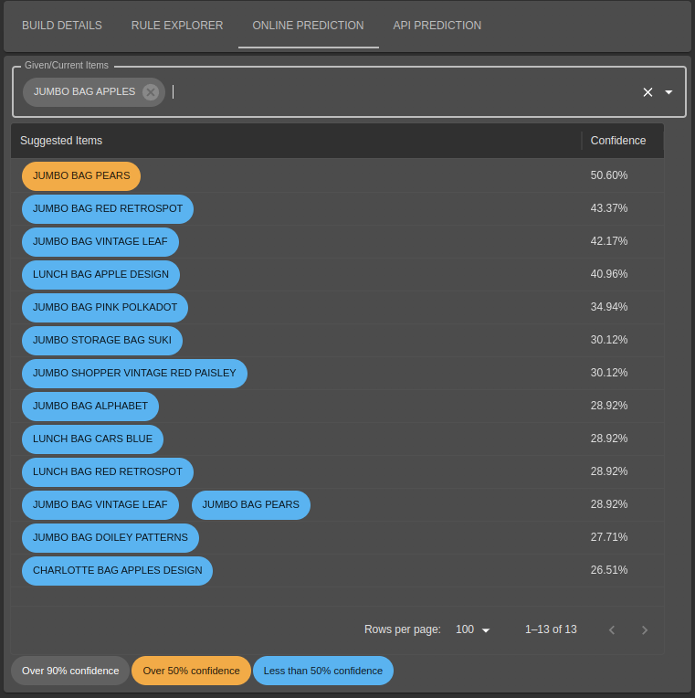
Online Prediction is backed by a highly-available, performant API you can use from your ERP, POS or other systems to make suggestions in real-time as orders are being created.
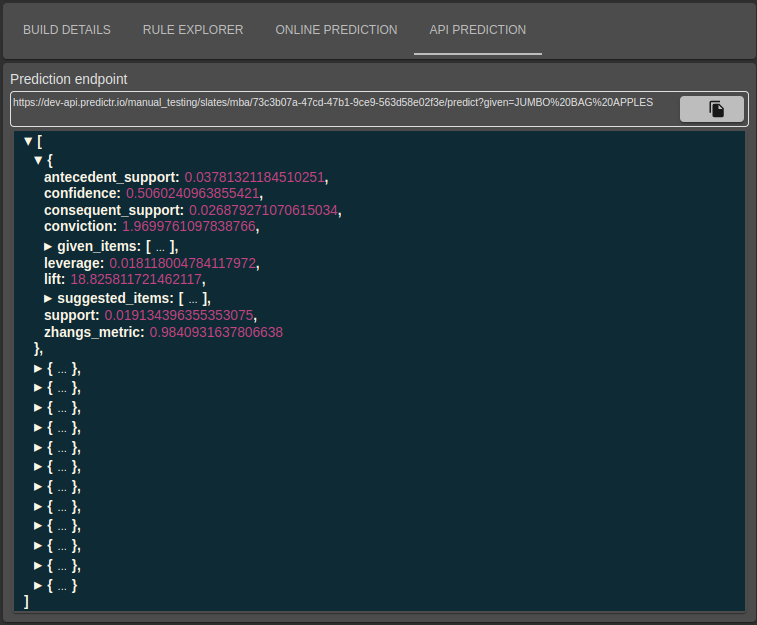
The API Prediction tab shows the API call equivalent to the items in the Online Prediction tab. See Using the API for more details on making automated predictions.